The paper titled “Probabilistic reasoning for streaming anomaly detection” from MIT CSAIL proposed a framework for performing online anomaly detection on univariate data. Unfortunately, most of the data in the real world are multivariate. Hence, mandating the need for more research into performing online anomaly detection in multivariate data. We have been inspired by their work and extend their framework to support multivariate data with some clever optimizations to build a scalable system.
### **Real-Life Impact of this Research**
+ This work has been published in the 31st ACM International Conference on Information and Knowledge Management, CIKM workshop titled [Applied Machine Learning Methods for Time Series Forecasting](https://ceur-ws.org/Vol-3375/), [pdf](https://ceur-ws.org/Vol-3375/paper6.pdf).
+ A startup founder confirmed to me that they successfully used my work in their production systems.
One might wonder why we have chosen this paper [[1]]() for our study. One answer to this question is that to the best of our knowledge, their work provided a simple framework based on basic statistics to perform real-time anomaly detection of a stream. Furthermore, during my master's thesis, I successfully used a derivation of their work for breaking news detection of an aggregated news stream. Another development that motivated this work is a challenge that I posed during my talk about [time series analysis](https://kenluck2001.github.io/blog_post/pysmooth_a_time_series_library_from_first_principles.html) in Vancouver. I asked the crowd if they can provide suggestions on how to adapt the presented solution to handle multivariate data streams. This is the result of that bet as it is an attempt to complete unfinished work.
The blog will begin by introducing the topic of anomaly detection, followed by a discussion of the original paper [[1]](), and describing extensions of the existing work to handle multivariate data streams. The novel formulation that we are proposing would depend on building an online version of the covariance matrix. As such, we have provided an implementation of the online covariance matrix, alongside an online inverse covariance matrix based on the Sherman-Morrison formula. We have provided a set of mathematical representations and source code.
My implementation of the original paper and the enhanced version of our modified algorithm which is the subject of this blog post can be found in the following links.
- Original paper code: https://github.com/kenluck2001/anomaly
- Blog code: https://github.com/kenluck2001/anomalyMulti
Furthermore, we have provided a set of detailed experiments on the proposed algorithms in different realistic scenarios. However, we maintain the statistical framework provided by the original [1]() paper as it has been tested. We will not fall into the trap of making this writing a survey paper. Hence, we will discuss a few interesting developments in space, and as such this manuscript is not expected to be exhaustive. This blog will focus on statistical models. As such, we won't discuss neural networks and their variants in any depth. This is becauseose would fall outside the scope of this blog post. For more information, see the [paper](https://arxiv.org/abs/1901.03407).
Anomaly detection is the task of classifying patterns that depict abnormal behavior. Therefore, the notion of normal behavior has to be quantified in some way. This concept can be described by several names such as outlier detection, novelty detection, noise detection, and deviation detection. These names are equivalent and would be used interchangeably for the remainder of our monograph. Outliers can arise as a result of human error, equipment error, and faulty systems. Anomaly detection is well-suited for unbalanced data, where the ideal scenario is to predict the behavior of the minority class. There are many applications of anomaly detection, such as detecting default on loans, fraud detection, and network intrusion detection among others.
There are [different types](http://cucis.ece.northwestern.edu/projects/DMS/publications/AnomalyDetection.pdf) of anomalies which are discussed as follows.
- Point anomaly: This is where a single instance is classified as an anomaly concerning the entire data set. This is ideal for univariate data.
- Contextual Anomaly: when a data instance can be anomalous based on the context (attributes and position in the stream) of the data. Such a method is ideal for multivariate data, where a single attribute of a snapshot reading may appear anomalous in a multivariate reading. However, it can be normal behaviour when considering the entire dataset.
- Collective anomalies are a collection of data points that exhibit anomalous behaviors as a group but exhibit normal behavior individually.
We have summarized many approaches for performing anomaly detection. Our categorization follows loosely the groupings described in [paper](http://citeseerx.ist.psu.edu/viewdoc/download?doi=10.1.1.109.1943&rep=rep1&type=pdf) to group existing approaches for anomaly detection
- Unsupervised: This is classifying an outlier with training on unlabelled data.
- Supervised: This is classifying an outlier with training on labeled data.
- Hybrid (mix of both): This is a mix of both schemes. These include semi-supervised learning, self-supervised learning e.t.c.
Anomaly detection algorithms can operate in many settings. This should be carefully thought out according to the problem at hand.
- Static: These algorithms are designed to work in static datasets. Every item is loaded into memory at a time to perform computation.
- Online: These algorithms are designed to work in real-time data streams. Items are incrementally loaded into memory.
- Static + Online: The model can operate in two stages. The initial parameters are estimated in the static setting. Once the parameters are set, as more data arrives, these parameters are incrementally updated. Similarly, our extensions and original work are of this type.
Our discussion will be incomplete if we don't describe how to maintain a collection of the data in the stream to be processed. Hence, we do a quick review of the windows. [Windows](https://www.kdd.org/exploration_files/20-1-Article2.pdf) provide a way to manage data streams. There are several window techniques for streaming analytics:
- Fixed window: This is using a fixed window to store some past information to allow for processing.
- Adaptive window (ADWIN): Keep two windows and drop the former if the past distribution deviates from the current distribution.
- Landmark window: Keep a history of data points that is representative of the distribution of the stream.
- Damped window: This intensifies or dampens the signal by weighting the most recent sample against the past sample. To forget the past, increase the weight of the present.
We have decided to work on anomaly detection algorithms that work in an unsupervised manner. The normal behavior is represented using the PDF of a multivariate normal distribution. Thresholds are set as a way to specify the significance level. The online formulation was used in our work to help the algorithm work even when concept drift occurs. Unsupervised learning provided advantages in cases where getting data with labels can be challenging or even impossible in some contexts. This fits nicely with a data stream when you don't know what to expect from your test distribution.
We will proceed to describe the algorithm in the original paper [[1]]() and then provide extensions in upcoming sections.
### Background work
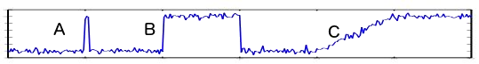
An anomaly detection algorithm automatically detects outliers in (a single or a combination of) the signal variations, which include an abrupt transient shift, an abrupt distributional shift, or a gradual distributional shift [[1]](), which is labeled as "A", "B", and "C", respectively.
Online algorithms are useful for real-time applications, as they operate incrementally, which is ideal for analyzing the data streams. These algorithms incrementally receive input and make a decision based on an updated parameter that conveys the current state of the data stream. This philosophy contrasts with offline algorithms that assume the entire data is available in memory. The issue with an offline algorithm is that the data must fit in memory. The online algorithm should be both time and space-efficient.
Anomaly detection algorithms may work in diagnosis or accommodation mode [[2]](). The diagnosis method identifies the outlier in the data for further processing of the outlier. The outlier is removed from the data sample, so it does not skew the distribution. This is useful when the exact parameters of the distribution are known, so the outlier is excluded from the further estimation of the parameters of the distribution [[2]](). The accommodation method identifies the outliers and uses them for estimating the parameters of the statistical model. This is suitable for data streams that account for the effect of concept drift [[3]]().
Exponential Weighted Moving Average (EWMA) is ideal for keeping a set of running moments in the data stream, but it has some limitations that have led the authors to introduce Probabilistic Exponentially Weighted Moving Average (PEWMA). A single slide from my presentation will clear every misconception between the two algorithms (EWMA and PEWMA) in context.
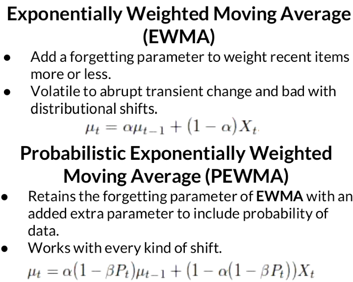
PEWMA [[1]]() algorithm operates in accommodation mode. The algorithm allows for concept drift [[3]](), which occurs in data streams, by updating the set of parameters that convey the state of the stream. PEWMA [[1]]() is suitable as an anomaly detection algorithm that works on an abrupt transient shift, where EWMA fails.
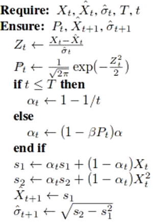
The parameters of the anomaly detection algorithm consist of $X_{t}$ the current data, $\mu_{t}$ the mean of the data, $\hat{X_{t}}$ is the mean of the data, $\hat{\alpha_{t}}$ the current standard deviation, $P_{t}$ the probability density function, $\hat{X_{t+1}}$ the mean of the next data (incremental aggregate), $\hat{\alpha_{t+1}}$ the next standard deviation (incremental aggregates), $T$ the data size, and $t$ a point in $T$. Initialize the process by setting the initial data for training the model $s_{1} = X_{1}$ and $s_{2} = X_{1}^{2}$.
The processed data is fed to the anomaly detection algorithm with the parameters $\alpha = 0.98, \beta = 0.98$, and $\tau = 0.0044$. The thresholds are chosen for determining outliers that are greater than 3 times the standard deviation in normally distributed data. PEWMA in the original paper was designed to work for point anomaly
##### Hypothesis Testing
A hypothesis is a subjective intuition about the problem. This can be guided by current best practices or transferable skills from adjacent domains. These forms of educated guesses have to be empirically verified to allow your preconceived intuitions to be checked against reality. Let us look at some examples of hypotheses:
- Will this vaccine work on a new virus?
- Will It rain today?
Let us look at the example of a certain school where the Physics teacher is generous with marks. The end-of-semester report has a class average of 80 with a standard deviation of 15. What is the probability that a student scores
- score < 60 ?
- score > 90 ?
The following code snippet solves the problem as a student scoring less than 60 and greater than 90 has a probability of 0.09 and 0.25 respectively.
```
import math
def cumfunc(mean, sigma, xval):
"""
@summary: cumulative pdf to the left of the standard normal distribution curve.
"""
z = (xval - mean) / (sigma * math.sqrt(2))
y = 0.5 * (1 + math.erf(z))
return y
if __name__ == '__main__':
mean = 80; sigma = 15
x = 60
res = cumfunc(mean, sigma, x) # < 60
print (round(res, 2)) # 0.09
x = 90
res = 1 - cumfunc(mean, sigma, x) # > 90
print (round(res, 2)) # 0.25
```
Let us provide the source code for visualizing the probability of the events described in the code snippet.
```
import numpy as np
import matplotlib.pyplot as plt
from scipy.stats import norm
def contour(plt, score, x_axis, y_axis, colour, lessthan=True):
x_temp = [x for x in x_axis if x <= score]
if lessthan:
y_temp = y_axis[:len(x_temp)]
else:
y_temp = y_axis[len(x_temp): ]
x_temp = [x for x in x_axis if x > score]
plt.fill_between(x_temp, 0, y_temp, facecolor=colour)
if __name__ == '__main__':
mean = 80; sd = 15
x_axis, y_axis = np.arange(10, 140, 0.001), norm.pdf(x_axis,mean,sd)
plt.plot(x_axis, y_axis); plt.xlabel('Scores'); plt.ylabel('PDF')
plt.title("Gaussian Distribution with Mean: {} and STD: {}".format(mean, sd))
colour='#4dac26'; score = 60
contour(plt, score, x_axis, y_axis, colour, lessthan=True)
colour='#f1b6da'; score = 90
contour(plt, score, x_axis, y_axis, colour, lessthan=False)
plt.show()
```
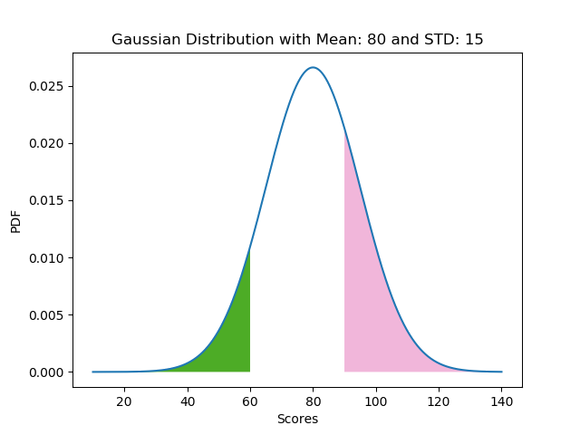
The probability of events (score < 60 and score > 90) is captured by the area of the shaded regions.
If the class average is 80 with a standard deviation of 15, it is a minuscule probability that a student scores less than 0 or greater than 120. The event with these outrageous scores can be said to be an anomaly. The scores used in our examples are thresholds. The areas depicting these probabilities can be seen in our chart.
In summary, the rule of thumb for hypothesis testing can be summarized as follows:
- Identify the Null and Alternative hypotheses.
- Choose a significance level by setting the threshold.
- Decide to reject based on the significance level.
### Extension
Our contribution begins here. We simplify the algorithm by ignoring the details of evolutionary computation in the [paper](http://www.cmap.polytechnique.fr/~nikolaus.hansen/ACECMUaa1p1CMAfES.pdf). The author of the blog post took the premise of evolution as described in the paper to be moving from one generation to the next; as equivalent to moving from one state to another state. This is analogous to how online algorithms work with dynamic changes as new data enters the stream. Cholesky decomposition is used extensively in the algorithms. The [paper](http://www.cmap.polytechnique.fr/~nikolaus.hansen/ACECMUaa1p1CMAfES.pdf) provided the basis for the online covariance matrix used in this work.
##### Online Covariance matrix
The mathematical formulation can be found here.
1. Estimate covariance matrix for initial data, $X \in R^{n \times m}$.
Initial covariance matrix, $C$ where $C \in R^{n \times m}$, $n$ is the number of samples, $m$ is the number of dimensions.
\begin{equation}
C = X * {X}^T
\end{equation}
2. Perform Cholesky factorization on the initial covariance matrix, $C$.
\begin{equation}
C_t = A_t * {A_t}^T
\end{equation}
We make use of Scipy's Cholesky decomposition. The input matrix must be positive-definite which means that the eigenvalues are positive which is a requirement for the Cholesky decomposition. For a quick primer on positive-definite, positive semi-definite, and their variants, peruse the [tutorial](https://www.cse.iitk.ac.in/users/rmittal/prev_course/s14/notes/lec11.pdf). The covariance matrix of a multivariate distribution is positive and semi-definite. For more insight on how to create a positive semi-definite covariance matrix. Kindly take a look at [discussion board](https://www.researchgate.net/post/How_to_generate_positive-definite_covariance_matrices). The approach taken in this work is to convert to the nearest positive definite matrix. This is sufficient for our purpose. Evaluate and adapt to your use case. A kind of reasonable approach is starting from a random positive definite matrix as a default choice for your covariance.
3. The general form of incremental covariance. It can be best understood that the updated covariance in the presence of new data is the weighted average of the past covariance without the new data and the covariance of the transformed input.
\begin{equation}
C_{t+1} = \alpha * C_t + \beta * v_t * {v_t}^T
\end{equation}
Where $v_t = A_t * z_t$ and $z_t \in R^m$ is understood in our implementation is the current data. \alpha and \beta are positive scalar values.
4. Update the Cholesky factor of the covariance matrix
\begin{equation}
A_{t+1} = \sqrt{\alpha} * A_t + \frac{\sqrt{\alpha}}{\Big\|z_t \Big\|^2} * \left( \sqrt{1 + \frac{\beta * \Big\|z_t \Big\|^2}{\alpha}} - 1 \right) * v_t * z_t
\end{equation}
5. There are difficulties with setting the values of $\alpha$ and $\beta$ respectively. $\alpha + \beta = 1$ as an explicit form of exponential moving average. The author chose to set the values of $\alpha$, and $\beta$ using the statistics of the data stream.
The parameters are set as $\alpha = {C_{a}}^2$, $\beta = 1 - {C_{a}}^2$ and $n$ is the size of the original data in the static settings.
Where ${C_{a}} = \sqrt{1 - C_{cov}}$ and $C_{cov} = \frac{2}{{n^2}+6}$.
\begin{equation}
A_{t+1} = {C_{a}} * A_t + \frac{{C_{a}}}{\Big\|z_t \Big\|^2} * \left( \sqrt{1 + \frac{(1 - {C_{a}}^2) * \Big\|z_t \Big\|^2}{{C_{a}}^2}} - 1 \right) * v_t * z_t
\end{equation}
The Implementation can be found here
```
def updateCovariance(alpha, beta, C_t, A_t, z_t):
"""
@param: alpha, beta, A_t are parameters of the model
@param: C_t is the old covariance matrix, z_t as the new data vector
@return: C_tplus1 is an updated covariance matrix
"""
v_t = np.dot(A_t, z_t.T)
C_tplus1 = (alpha * C_t) + (beta * np.matmul(v_t, v_t.T))
print ("v_t: {}, C_tplus1: {}".format(v_t.shape, C_tplus1.shape))
return C_tplus1
def updateCholeskyFactor(alpha, beta, A_t, z_t):
"""
@param: alpha, beta, A_t are parameters of the model
@param: z_t as a new data vector
@return: A_tplus1 is an updated covariance matrix
"""
v_t = np.dot(A_t, z_t.T)
norm_z = np.linalg.norm(z_t)
x = math.sqrt(alpha) * A_t
w = beta * norm_z / alpha
y = math.sqrt(alpha) * (math.sqrt(1 + w) - 1) * np.dot(v_t, z_t) / norm_z
A_tplus1 = x + y
print ("A_t: {}, A_tplus1: {}".format(A_t.shape, A_tplus1.shape))
return A_tplus1
```
##### Online Inverse Covariance matrix
The mathematical formulation can be found here
1. Estimate covariance matrix for initial data, $X \in R^{n \times m}$.
Initial covariance matrix, $C$ where $C \in R^{n \times m}$, $n$ is the number of samples, $m$ is the number of dimensions.
\begin{equation}
C = X * {X}^T
\end{equation}
Inverse the covariance matrix, $C^{-1}$.
\begin{equation}
C^{-1} = \left( X * {X}^T \right)^{-1}
\end{equation}
2. Perform Cholesky factorization on the initial covariance matrix, $C$.
\begin{equation}
C_t = A_t * {A_t}^T
\end{equation}
3. General form of incremental covariance.
It is best understood that the updated covariance in the presence of new data is equivalent to the weighted average of the previous covariance without the new data and the covariance of the transformed input.
\begin{equation}
C_{t+1} = \alpha * C_t + \beta * v_t * {v_t}^T
\end{equation}
Where $v_t = A_t * z_t$ and $z_t \in R^m$ is understood in our implementation is the current data. \alpha and \beta are positive scalar values.
4. Update the Cholesky factor of the covariance matrix
\begin{equation}
C_{t+1}^{-1} = (\alpha * C_t + \beta * v_t * {v_t}^T)^{-1}
\end{equation}
\begin{equation}
C_{t+1}^{-1} = \alpha^{-1} * (C_t + \frac{\beta * v_t * {v_t}^T}{\alpha})^{-1}
\end{equation}
Let us fix, $\hat{v_t} = \frac{\beta * v_t}{\alpha}$. The resulting simplification using Sherman-Morrison Formula reduces the expression to
\begin{equation}
C_{t+1}^{-1} = \frac{1}{\alpha} * \left({{C_t}^{-1}} - \frac{{{C_t}^{-1}} * \hat{v_t} * {v_t}^T * {{C_t}^{-1}}}{1 + (\hat{v_t} * {{C_t}^{-1}} * {v_t}^T)} \right)
\end{equation}
The Implementation can be found here
```
def updateInverseCovariance(alpha, beta, invC_t, A_t, z_t):
"""
@param: alpha, beta, A_t are parameters of the model
@param: invC_t is the old inverse covariance matrix, z_t as a new data vector
@return: invC_tplus1 is an updated inverse covariance matrix
"""
print ("A_t: {}, z_t: {}".format(A_t.shape, z_t.shape))
v_t = np.dot(A_t, z_t.T)
hat_vt = (beta * v_t) / alpha
print ("invC_t: {}, hat_vt: {}, v_t: {}, invC_t: {}".format(invC_t.shape, hat_vt.shape, v_t.shape, invC_t.shape))
y = multi_dot([invC_t, hat_vt, v_t.T, invC_t]) / (1 + multi_dot([hat_vt.T, invC_t, v_t]))
invC_tplus1 = (invC_t - y) / alpha
print ("invC_tplus1: {}".format(invC_tplus1.shape))
return invC_tplus1
```
##### Online Multivariate Anomaly Detection
The probability density function is based on ideas from hypothesis testing. We decide on a threshold which is a confidence level that is used to decide on the acceptance and rejection regions.
1. Use the covariance matrix, $C_{t+1}$ and inverse covariance matrix, ${C_{t+1}}^{-1}$.
2. However, we attempt to increment the mean vector, $\mu$ as new data arrives. It is possible to simplify the Covariance matrix, $C$, which will capture a number of the dynamics of the system. Let $n$ represent the current count of data before new data has arrived.
Also, $\hat{x}$: is the new data, $\mu_{t+1}$: moving average
\begin{equation}
\mu_{t+1} = \frac{(n * \mu_t) + \hat{x}}{n+1}
\end{equation}
3. Set a threshold to determine the acceptance and rejection regions. Items in the acceptance region are considered to be normal behavior.
\begin{equation}
p(x)=\frac{1}{\sqrt{(2\pi)^m|C|}} \exp\left(-\frac{1}{2}(x-\mu)^T{C}^{-1}(x-\mu) \right)
\end{equation}
Where $\mu$ is mean vector, $C$ is covariance matrix, $|C|$ is the determinant of $C$ matrix, $x \in R^{m}$ is data vector, and $m$ is the dimension of $x$ respectively.
The Implementation can be found here
```
def anomaly(x, mean, cov, threshold=0.001):
"""
@param: x is the current data vector
@param: mean is the mean vector
@param: cov is a covariance matrix
@return: score
"""
score = multivariate_normal.pdf(x, mean=mean, cov=cov)
return score
def updateMean(mean, z):
mean_tplus1 = ((n * mean) + z) / (n + 1)
return mean_tplus1
```
We have provided a clean object-oriented programming-based solution with a cleaner API.
```
seed = 0
np.random.seed(seed)
X = np.random.rand(1000,15)
z_t0 = np.random.rand(1,15) # new data
# single case predict
anom = probabilisticMultiEWMA()
anom.init(X)
z_t0 = np.random.rand(1,15) # new data
anom.update(z_t0)
z_t1 = np.random.rand(1,15) # next new data
print ("score: {}".format(anom.predict(z_t1)))
Z = np.random.rand(1000,15)
# Bulk predict
anom = probabilisticMultiEWMA()
anom.init(X)
pred = anom.bulkPredict(Z)
print (pred)
```
### Experiments
A simulation of 10000000 vectors with dimensions of 15 was created to evaluate the usefulness of our algorithm. The repeated trial shows that our algorithm is not sensitive to initialization seeds and dimensions of the matrix. This requirement was a deciding factor in the choice of the evaluation metric. More information on the metric will be provided in the Discussion section.
This is to find the trade-off between the static window and the update window. The source code for the experiments can be found [here](https://github.com/kenluck2001/anomalyMulti/blob/master/normal_distribution_charts_with_example.py).
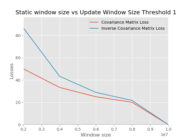
##### Experiment 1
The goal of this experiment is to check the effect of varying the size of the initial static window versus the update window
Generally, the experiment setup follows the description.
- Split the data into 5 segments
train on 1st segment(static), update covariance on 2nd (online), compare with static covariance - get error
- Train on 1, 2 segment(static), update covariance on 3rd (online), compare with static covariance - get error.
- Train on 1, 2, 3 segment(static), update covariance on 4th (online), compare with static covariance - get error
- Train on 1, 2, 3, 4 segment(static), update covariance on 5th (online), compare with static covariance - get error
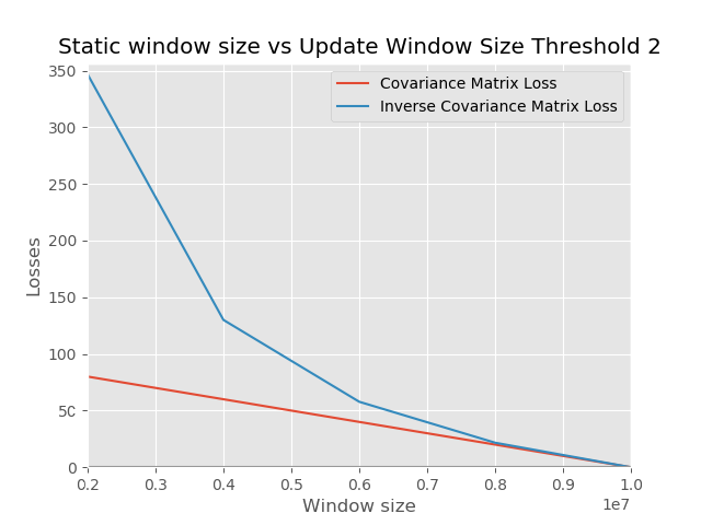
##### Experiment 2
The goal of this experiment is to check the effect of varying the size of the initial static window versus the update window
The experiment setup follows loosely the description
- Split the data into 5 segments.
- Train on 1st segment(static), update covariance on remaining segments (2,3,4,5) (online), compare with static covariance - get errors on segments (2,3,4,5)
- Train on 1, 2 segment(static), update covariance on remaining segments (3,4,5) (online), compare with static covariance - get errors on segments (3,4,5)
- Train on 1, 2, 3 segment(static), update covariance on remaining segments (4,5) (online), compare with static covariance - get errors on segments (4,5)
- Train on 1, 2, 3, 4 segment(static), update covariance on remaining segments (5) (online), compare with static covariance - get errors on segments (5)
### Discussion
Our matrix was flattened to a vector which is passed as input. The length of the vector is used to compute the loss metric that is agnostic to the dimension of the matrix. The loss function used in the evaluation is Absolute Average Deviation (AAD) because it gives a tighter bound on the error in comparison to MSE or MAD. This is because we take the average of the residuals divided by the ground truth for every sample in our evaluation set. If the residual is close to zero, we contribute almost nothing to the measure. However, if the residual is large, we want to know the factor that makes it large in comparison to the ground truth. This behavior of scaling by the ground truth may explain why this metric tends to be conservative in regression analysis.
\begin{equation}
AAD = \sum_{i=1}^{n} \left| \frac{\hat{Y_i} - Y_i}{Y_i} \right|
\end{equation}
Where $\hat{Y_i}$ is the predicted value, $Y_i$ is the ground truth, and $n$ is the length of the flattened matrix.
From our experiments, we can see that building your model with more data in the init (static) phase tends to lead to smaller errors in comparison to having smaller data in the init phase and using more of the data for an update. The observation is in line with what we expect because when you operate in an online mode, you tend to use less storage space. However, the performance sacrifice is lower than when you operate in batch mode.
The error at the beginning of our training is huge in both charts. This insight shows that rather than performing the expensive operation of converting a covariance matrix to have the property of positive definiteness, it is better to just use random matrices that are positive definite. More data would help us achieve convergence as more data arrives.
There are many challenges with anomaly detection methods in modeling the normal behavior of the system. The abnormal behavior shows a deviation from what is expected to be the normal behavior of the system. Many anomaly detections are susceptible to adversarial attacks. In a supervised setting, getting labeled data can be expensive. The definition of noise can be ambiguous.
As a result of the successful experiments, we are confident that we will experience similar outcomes to the univariate case described in the original paper. As a result, we will enhance our support for multivariate cases.
### Conclusion
There is no generic anomaly detection that works for every possible task. It has to be tuned for your purpose. The underlying assumption in this work is that the features that are used capture significant information about the underlying dynamic of the system. Future work can include extending the multivariate version of the anomaly algorithm to be production-ready.
Spoiler alert: Some of the contents here are lifted verbatim from my master's thesis.
### Acknowledgements
I would like to thank my mentor, Dr. Ziyuan Gao from the National University of Singapore for providing technical support during the writing of this manuscript.
### References
- [[1]]() Kevin M. Carter and William W. Streilein. Probabilistic reasoning for streaming anomaly detection. In Proceedings of the Statistical Signal Processing Workshop, pages 377–380, 2012.
- [[2]]() Victoria Hodge and Jim Austin. A survey of outlier detection methodologies. Artificial Intelligence Review, 22(2):85–126, 2004.
- [[3]]() Gregory Ditzler and Robi Polikar. Incremental learning of concept drifts from streaming imbalanced data. IEEE Transactions on Knowledge and Data Engineering, 25(10):2283–2301, 2013.
### **How to Cite this Article**
```
BibTeX Citation
@article{kodoh2020,
author = {Odoh, Kenneth},
title = {Real-Time Anomaly Detection for Multivariate Data Stream},
year = {2020},
note = {https://kenluck2001.github.io/blog_post/real-time_anomaly_detection_for_multivariate_data_stream}
}
```
11/18
Please feel free to donate to support my work by clicking